数据来源 https://www.kaggle.com/datasets/masoudnickparvar/brain-tumor-mri-dataset
导入库 1 2 3 4 import tensorflow as tf from tensorflow import keras from tensorflow.keras import layers from tensorflow.keras.applications.densenet import preprocess_input
检查是否启用了GPU 1 print (tf.config.list_physical_devices("GPU" ))
[PhysicalDevice(name=’/physical_device:GPU:0’, device_type=’GPU’)]
构造数据集 1 2 3 4 5 6 7 8 9 10 11 12 13 14 15 16 17 18 19 20 21 22 23 BATCH_SIZE = 32 IMG_SIZE = (224, 224) DATA_DIR = "/Volumes/HIKSEMI/ipynb/Kaggle/Brain Tumor Dataset" train_ds_raw = tf.keras.preprocessing.image_dataset_from_directory( DATA_DIR, validation_split=0.2, subset="training" , seed=123, color_mode="rgb" , image_size=IMG_SIZE, batch_size=BATCH_SIZE, ) val_ds_raw = tf.keras.preprocessing.image_dataset_from_directory( DATA_DIR, validation_split=0.2, subset="validation" , seed=123, color_mode="rgb" , image_size=IMG_SIZE, batch_size=BATCH_SIZE, )
Found 10560 files belonging to 4 classes.
1 2 3 4 5 6 7 class_names = train_ds_raw.class_names num_classes = len(class_names) print ("类别:" , class_names)AUTOTUNE = tf.data.AUTOTUNE train_ds = train_ds_raw.cache().shuffle(1000).prefetch(buffer_size=AUTOTUNE) val_ds = val_ds_raw.cache().prefetch(buffer_size=AUTOTUNE)
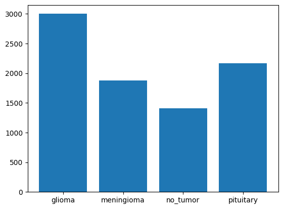
查看不同标签图片的数量 1 2 3 4 5 6 7 import numpy as np import matplotlib.pyplot as plt counts = np.bincount([y for x, y in train_ds.unbatch()]) plt.bar(range(len(class_names)), counts) plt.xticks(range(len(class_names)), class_names) plt.show()
数据增强 1 2 3 4 5 6 7 8 9 IMG_SIZE = (224, 224) data_augmentation = tf.keras.Sequential([ layers.RandomFlip("horizontal_and_vertical" ), layers.RandomRotation(0.15), layers.RandomZoom(0.2), layers.RandomContrast(0.2), layers.RandomBrightness(0.2) ])
模型选择 1 2 3 4 5 6 7 8 9 10 11 12 13 14 15 16 17 base_model = tf.keras.applications.DenseNet121( include_top=False, weights='imagenet' , input_shape=(224, 224, 3) ) base_model.trainable = False model = models.Sequential([ data_augmentation, layers.Lambda(preprocess_input), base_model, layers.GlobalAveragePooling2D(), layers.Dropout(0.3), layers.Dense(128, activation='relu' , kernel_regularizer=tf.keras.regularizers.l2(1e-4)), layers.Dense(4, activation='softmax' ) ])
迁移学习 第一阶段 1 2 3 4 5 6 7 8 9 10 11 12 13 14 15 16 model.compile( optimizer=tf.keras.optimizers.Adam(1e-3), loss='sparse_categorical_crossentropy' , metrics=['accuracy' ] ) print ("第一阶段" )history1 = model.fit( train_ds, validation_data=val_ds, epochs=10, callbacks=[ tf.keras.callbacks.EarlyStopping(monitor='val_loss' , patience=3, restore_best_weights=True) ] )
Epoch 1/10
第二阶段 1 2 3 4 5 6 7 8 9 10 11 12 13 14 15 16 17 18 19 20 21 22 23 24 25 26 27 28 29 30 31 32 33 34 base_model.trainable = True for layer in base_model.layers[:-80]: layer.trainable = False print (f"第二阶段" )print (f"可训练参数: {sum([tf.size(v).numpy() for v in model.trainable_variables])}" )model.compile( optimizer=tf.keras.optimizers.Adam(1e-5), loss='sparse_categorical_crossentropy' , metrics=['accuracy' ] ) callbacks = [ tf.keras.callbacks.EarlyStopping( monitor='val_loss' , patience=5, restore_best_weights=True ), tf.keras.callbacks.ReduceLROnPlateau( monitor='val_loss' , factor =0.5, patience=3, min_lr=1e-7 ) ] history2 = model.fit( train_ds, validation_data=val_ds, epochs=40, callbacks=callbacks )
…
验证 1 2 val_loss, val_acc = model.evaluate(val_ds_raw) print (f"验证集准确率: {val_acc:.3f}" )
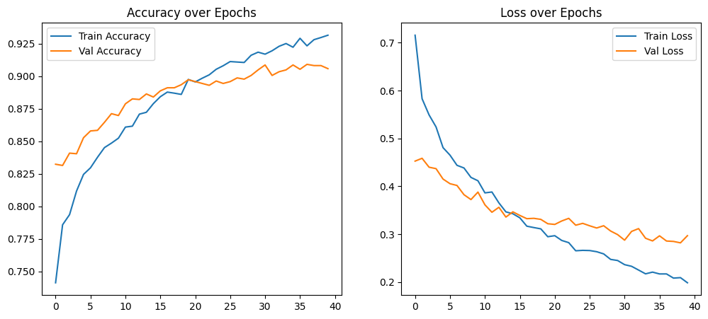
1 2 3 4 5 6 7 8 9 10 11 12 13 14 15 16 17 18 19 import matplotlib.pyplot as plt plt.figure(figsize=(12, 5)) plt.subplot(1, 2, 1) plt.plot(history2.history["accuracy" ], label="Train Accuracy" ) plt.plot(history2.history["val_accuracy" ], label="Val Accuracy" ) plt.legend() plt.title("Accuracy over Epochs" ) plt.subplot(1, 2, 2) plt.plot(history2.history["loss" ], label="Train Loss" ) plt.plot(history2.history["val_loss" ], label="Val Loss" ) plt.legend() plt.title("Loss over Epochs" ) plt.show()
保存模型 1 2 model.save("brain_tumor_model_3.keras" ) print ("模型已保存为 brain_tumor_model_3.keras" )
加载模型 1 2 3 4 model = tf.keras.models.load_model( "brain_tumor_model_3.keras" , custom_objects={"preprocess_input" : preprocess_input} )
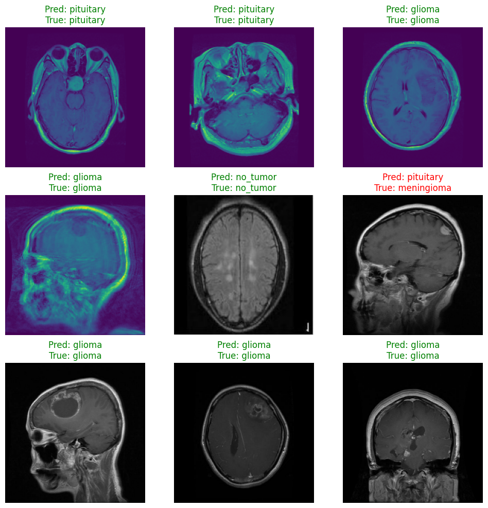
测试 1 2 3 4 5 6 7 8 9 10 11 12 13 14 15 16 17 18 19 import numpy as np import matplotlib.pyplot as plt class_names = train_ds_raw.class_names for images, labels in val_ds_raw.take(1): preds = model.predict(images) pred_labels = np.argmax(preds, axis=1) plt.figure(figsize=(12, 12)) for i in range(9): plt.subplot(3, 3, i + 1) plt.imshow(images[i].numpy().astype("uint8" )) true_label = class_names[labels[i]] pred_label = class_names[pred_labels[i]] color = "green" if true_label == pred_label else "red" plt.title(f"Pred: {pred_label}\nTrue: {true_label}" , color=color) plt.axis("off" ) plt.show()
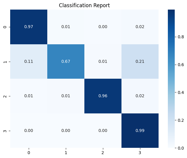
分类报告 1 2 3 4 5 6 7 8 9 10 11 12 13 14 15 16 17 18 19 20 21 22 23 24 25 26 27 28 29 30 import numpy as np import matplotlib.pyplot as plt import seaborn as sns from sklearn.metrics import confusion_matrix, classification_report y_true = [] y_pred = [] for images, labels in val_ds: preds = model.predict(images, verbose=0) preds_class = np.argmax(preds, axis=1) y_true.extend(labels.numpy()) y_pred.extend(preds_class) y_true = np.array(y_true) y_pred = np.array(y_pred) print ("Classification Report:" )print (classification_report(y_true, y_pred, digits=4))cm = confusion_matrix(y_true, y_pred) cm_norm = cm.astype('float' ) / cm.sum(axis=1)[:, np.newaxis] plt.figure(figsize=(8,6)) sns.heatmap(cm_norm, annot=True, fmt =".2f" , cmap="Blues" , cbar=True) plt.title("Classification Report" ) plt.show() val_acc = np.mean(y_true == y_pred) print (f"验证集准确率: {val_acc:.4f}" )